Economic, Enviromental & Other Influencing Factors of COVID-19 Deaths: Within Low-Income Countries
My first data science project looking at factors influencing COVID-19 deaths in low-income countries, using R Studio.

One of my first assignments for my MSc in Data Science was to write a 3000 word report describing how I explored and analysed data for a selected topic utilising the Our World in Data COVID-19 Dataset within R Studio (for full R Code see very bottom of post).
I decided to look into factors affecting low income countries as most of the news and media I consumed during the pandemic covered higher income countries. I was curious as to what was happening in other countries without our infrastrucutres, health care systems and access to technology.
This report ended up being 2982 words long (including references, appendices and words in tables/diagrams it actually came to a whooping 8044!). To save you time and a headache I've included summaries of the main sections. This assignment was graded a distinction and was my first data science project in academia and I am very proud of it despite its flaws.
Method(s):
Utilising publicly available datasets and the R software package. A multiple linear regression analysis of selected variables from the World Bank WDI (World Development Indicators) and Our World in Data COVID-19 datasets was performed, on countries defined by the World Bank as low-income. To find which variables had a significant influence on the total deaths per million. The Shapiro Wilks Test was implemented to statistically test the distribution of each variable. Log transformation was used for variables which did not satisfy p > 0.05. To check for any collinearity amongst the variables, a co-variance table utilising Spearman’s rank correlation coefficient was produced.
Why use total deaths per million and not another metric?
Other studies have used the CFR as their dependent variable however in this study the dependent variable chosen was TDPM due to several critiques of the CFR being used as a measure. CFR is calculated as: no. confirmed deaths/no. confirmed cases x 100 = mortality rate, highlighting two potential issues using this as a measure of COVID-19’s impact across countries:
1) CFR is based on number of “confirmed cases” and due to insufficient testing many cases are not confirmed (Gupta, M., Wahl, B., Adhikari, B. et al. , 2020; Hannah Ritchie et al., 2021)
2) CFR reflects the occurrence of COVID-19 at a particular point in time and is subject to change, therefore making it sensitive to location and population characteristics (Abel Brodeur et al., 2021) e.g. how a country classifies a COVID-19 death, socio-demogrpahic factors.
Why use the Shapiro Wilks test?
The results of the Shapiro Wilks test are not affected by scale and hence it is an appropriate test of the hypothesis of normality (Shapiro & Wilk, 1965).
The Shapiro Wilks test was chosen over other methods such as the Kolmogorov-Smirnov test and Anderson-Darling test as the sample size was < 30, the method used can be applied to small samples (n < 20). A drawback of the test is that for larger sample sizes (n>100) it may be difficult to approximate the values of multipliers in the numerator (Shapiro & Wilk, 1965).
(In a nutshell the shapiro wilks test is better for smaller samples!)
Stage 1: Data Gathering
Utilizing publicly available datasets for ease of access and less barriers to entry for study replication, this study is founded upon two large datasets:
1) Our World in Data (OWID) COVID-19 Dataset - Comprehensive time series dataset showing a variety of variables associated with COVID-19. Certain variables are updated either daily, weekly, or fixed. File type: .csv.
2) The World Bank, World Development Indicators (WDI) R Dataset - Compilation of international statistics regarding global/societal development and poverty of 266 countries. With 1443 time series indicators/variables, some with data going back more than 50 years. File type: .XML (downloaded from world banks API).
In the full report I provided a table that divided the variables by there category (Economic, Enviromental & Other), variable name, abbreviation, description, unit and source.
Stage 2: Data Structuring
The aforementioned two large datasets were refined into several smaller datasets for appropriate structure to be prepared for analysis. The diagram below shows this process, imagine it as the “flow of data”. Names in brackets denotes the names these data frames were given in the R environment.
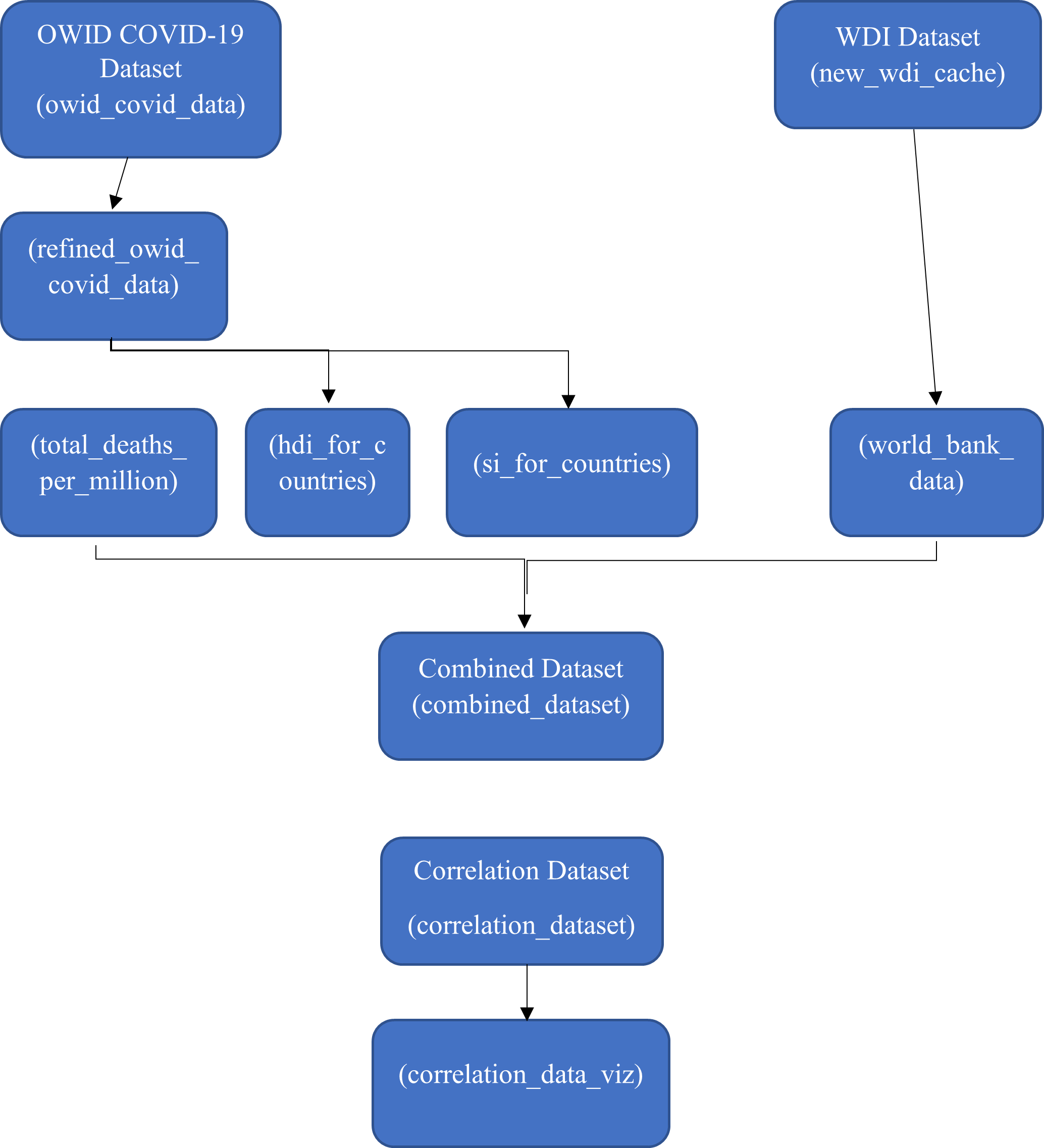
Note: si_for_countries
For the si_for_countries data frame an average of each countries stringency index (What does stringecy index mean?) from 01/01/2020 – 13/12/2021 was taken to give a representative figure of their governments stringency during this time period. As the stringency index variable included in the OWID COVID-19 is measured across time (daily) it was essential to convert this to a cross sectional figure which would represent it. Wary that it would not be an accurate measure of the countries stringency over time as it does not account for responsiveness of policy implementation across time. From this point on where “Stringency Index” is referred to this is referring to this average described.
Within the full report I included a dataframe(s) details table showing the dataframe, description and use. Data examples were given for each of the aforementioned dataframes to give readers samples of what the data looked like.
Stage 3: Exploratory Data Analysis (EDA)
Most of the Data Exploring/Analysis (EDA) was performed on the two data frames combined_dataset and correlation_dataset.
Descriptive statistics were observed to identify outliers within each variable list and to get a general overview of the data see the table below:

As part of the EDA, histograms were plotted to observe the distribution of the data graphically, this should be done to get a feel for the data and become familiar with it (O'Neil & Schutt, 2014)
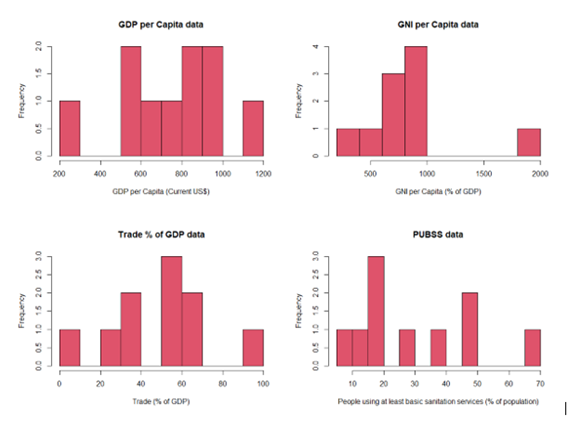
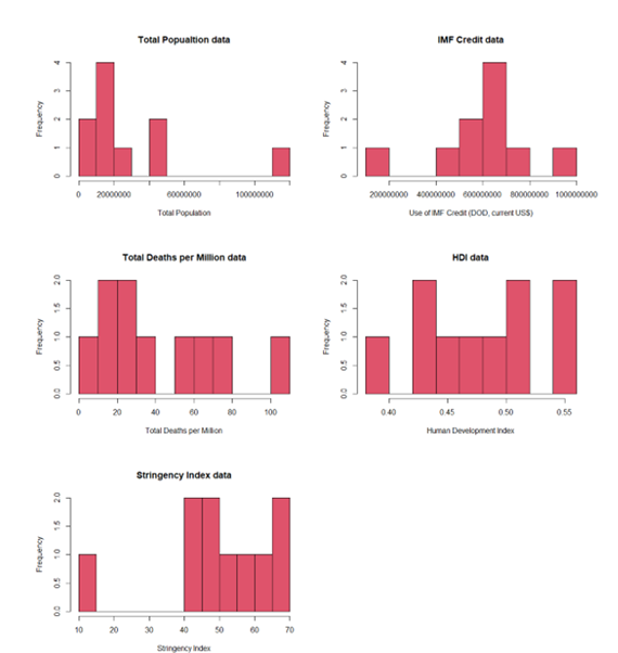
Further EDA
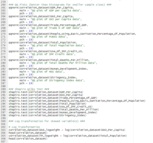
Quantile-Quantile (QQ) plots were also created to give a further visual representation if the data came from a theoretical distribution such as a normal or exponential distribution. But for the purpose of keeping this blog relatively short I have not included images of these.
A Shapiro Wilks test was employed to statistically test the distribution of the variables and not just solely rely on visual observation. A Shapiro Wilks test is obtained “by dividing the square of an appropriate linear combination of the sample order statistics by the usual symmetric estimate of variance.” (Shapiro & Wilk, 1965).
Null hypothesis: The data is normally distributed. If p > 0.05, the normality can be assumed.
See table below for the results of the test (values marked with * failed null hypothesis)
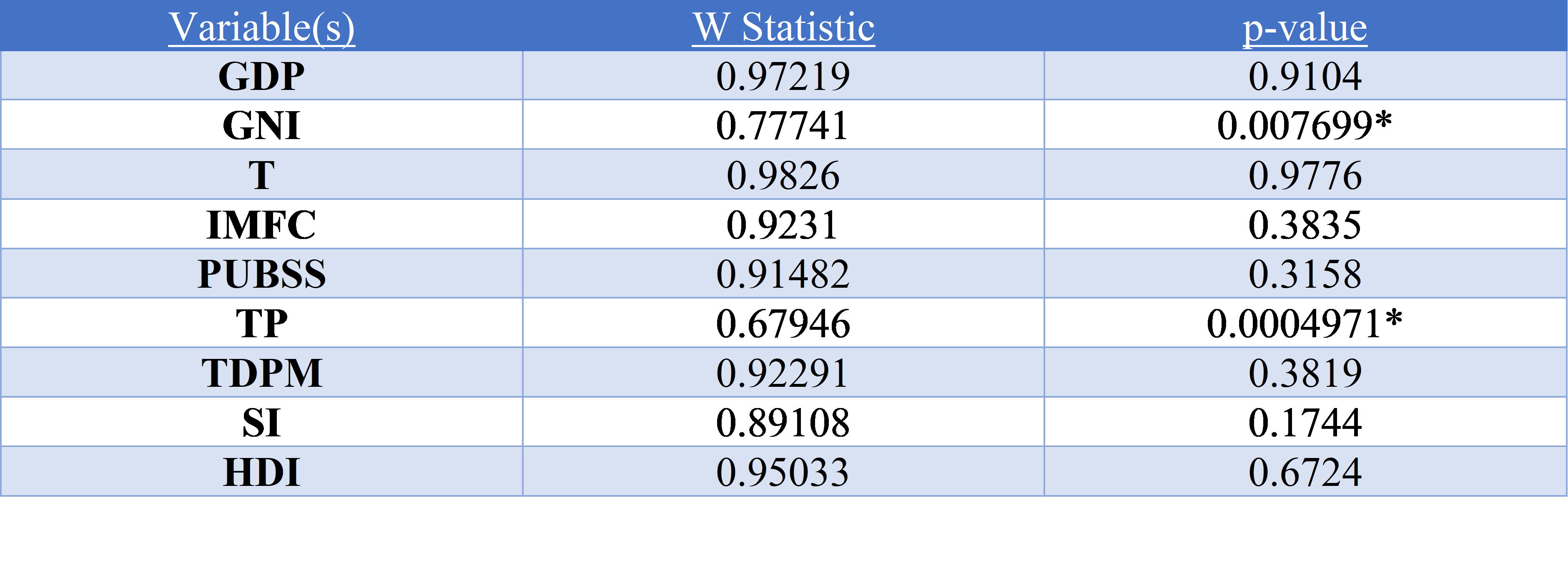
As highlighted in the table above the variables Gross National Income per Capita and Total Population failed the null hypothesis suggesting that they were not normally distributed, it is clear that the independent variables would have to be log transformed.
What is Log Transforming?
Log transforming the variables pulls in big values from the variable data and normalizes the variance across the observations of a variable
The base log function was used in R, which uses the mathematical constant, Euler’s number (ⅇ = 2.718282) as the base. The following lines of code produced two new log transformed versions of the variables which did not satisfy the null hypothesis:

Then the log transformed variables were then tested again for normality with the Shapiro Wilks test to see if they satisfied the null hypothesis (see results below).

These now satisfy the null hypothesis, proceeding with the EDA process and preforming the multiple linear regression analysis (MLR). But first, collinearity of independent variables must be checked.
What is Collinearity?
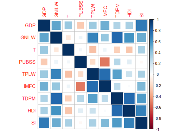
Collinearity refers to the phenomena when two of the explanatory variables are highly correlated, which may in turn make the MLR model unstable (Tranmer, Murphy, Elliot, & Pampaka, 2020).
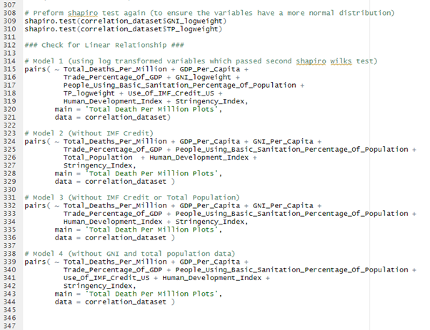
Spearman correlation rank was chosen to test the correlation over Pearson’s, due to the monotonic relationship between the variables and their ordinal nature (Rebekic, Loncaric, Petrovic, & Maric, 2015). Resulting in the correlation matrix below:
Now finally time for the crux of the biscuit... preforming the multiple linear regression.
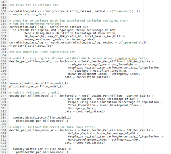
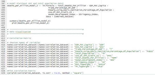
The method of least squares is used to estimate the regression coefficients in the MLR equation, these coefficients illustrate the contribution each independent variable has of predicting the dependent variable (Brown, 2009). Regression using more than one independent variable is referred to as a multivariate regression analysis (Tabachnick & Fidell, 1996). The model in R would be represented as these lines of code:

In the full report I then produced a methodology table (which was 11 pages long!!!) detailing the R packages used, functions and there use and justification, at each stage of the data science process.
Limitations and Weaknesses (There's a lot...)
As the CFR was earlier critiqued the TDPM is also a measure that is critiqued as different countries have different methods of classifying what counts as a COVID-19 death, ergo this will mean countries will report different amounts of deaths for their population depending on reporting methods (Hannah Ritchie et al., 2021). A universal measure of what counts as a COVID-19 death would solve this issue, for example in Canada total death figures include deaths from other causes “with” COVID-19 and in Italy no clinical diagnosis was needed following WHO definition or guidelines (Covid-19 Health System Response Monitor, 2022).
The traditional approaches of “simple statistics” including principal component analysis (PCA), clustering and single/multiple regression have been used throughout epidemiological studies to study the influence of independent variables on a dependent variable (Sannigrahi, Pilla, Basu, Basu, & Molter, 2020). This is also providing that that samples used in these models are independent of each other (Kauhl, et al., 2015). This study has not considered the spatial dependency of the independent variables of one another. As (Kauhl, et al., 2015) suggest when studying infectious diseases across large areas, spatial epidemiological methods may provide more insight when identifying hotspots, demographic and socio-economic determinants. Given more time this study would have incorporated spatial regression models (SRM), including as suggest by (Sannigrahi, Pilla, Basu, Basu, & Molter, 2020): spatial lag model (SLM), Spatial error model (SEM) and geographically weighted regression (GWR). This would consider the spatial auto correlation amongst the variables used in this study.
Stepwise regression was not used to select variables, taking the form of forward or backward sequence of F-tests or t-tests, however there are several critiques of this method. With respect to the domain of data mining, models created by this method may be oversimplifications of the real models of the underlying data (Roecker, 1991). Also, variables differ due to heterogeneous socio-economic characteristics which will affect the linearity of them and also distribution (Stojkoski, Utkovski, Jolakoski, Tevdovski, & Kocarev, 2020).
With more time it would be possible to quantify how long the country had been in the pandemic as demonstrated by (Stojkoski, Utkovski, Jolakoski, Tevdovski, & Kocarev, 2020) in this study, two variables were used to “quantify the possibility that countries are in a different state of the disease spreading process” (Stojkoski, Utkovski, Jolakoski, Tevdovski, & Kocarev, 2020). First variable: the number of days since the first registered case, second variable: evaluate the time which the country had to prepare for the first wave of coronavirus. “This is given as the number of days between the first registered case worldwide and the first case in the country.” (Stojkoski, Utkovski, Jolakoski, Tevdovski, & Kocarev, 2020).
Also, it is worth noting the values produced by the log transformation in section 2.3 are not the actual values of the variables and would have affected the model, even though they satisfy the assumption that all variables are normally distributed. With naturally occurring data this is common to find.
Stage 4: Results and Discussion
The results of the multiple linear regression model are presented below:
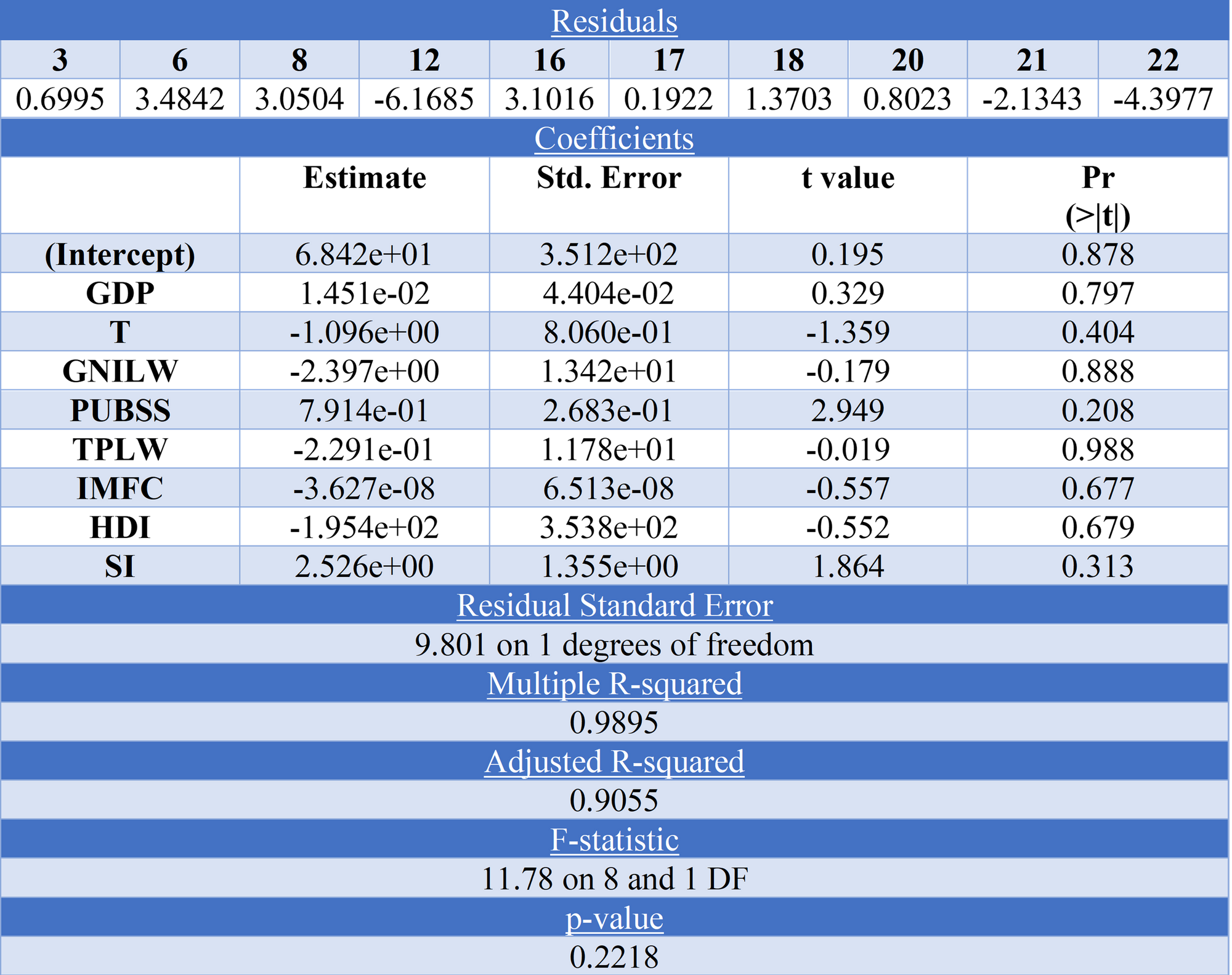
Here we can see that none of the independent variables are statistically significant, however out of the variables measured the most influential on total deaths per million were: T (Total population), PUBSS (People using basic sanitation services) and SI (Stringency Index).
As for the Beta coefficients GDP was positive at 1.451e-02 showing that an increase in GDP would mean an increase in TDPM, this was also demonstrated by (Abel Brodeur et al., 2021), finding that more economically developed countries had more cases/deaths but this could be due to more testing capabilities (Gupta, M., Wahl, B., Adhikari, B. et al. , 2020). Total population was negative at -1.096e+00, which would make sense as with less population naturally there will be less deaths (if all population characteristics and demographics stayed the same). PUBSS was positive at 7.914e-01 which may be a reflection of the former point as with more economic development more of the population uses basic sanitation, but initially one would expect access to basic sanitation to decrease the chance of death from infectious diseases, as unsafe sanitation is a leading risk factor in deaths related to infectious diseases (Our World In Data, 2022). SI was positive at 2.526e+00 which is supported by the literature that government interventions around the world had some impact on reducing COVID-19 deaths (Abel Brodeur et al., 2021).
Conlusion
Although none of the variables were statistically significant/influential on the TDPM, this study highlights some areas which may need closer attention and further study. It successfully contributes to the lack of research in low-income countries as formally mentioned by (Jay J H Park et al., 2021). By doing so, and with a clear methodology this may lead to more research with the same model but different independent variables. With more time and resources more variables could have been considered within multiple models.
Key points
· More research is needed within low-income countries regarding COVID-19 and its causes and effects.
· With a clear methodology this study provides a framework that can be repeated so further studies can be performed.
· Although no statistically significant independent variables were found the most influential on the model were Total Population, People Using Basic Sanitation Services and Stringency Index.
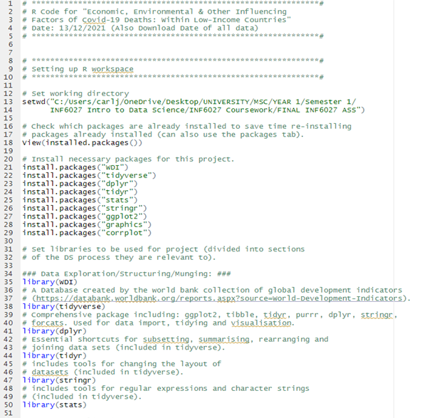
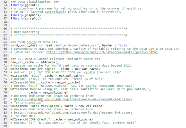
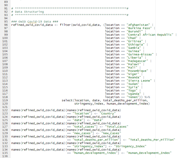
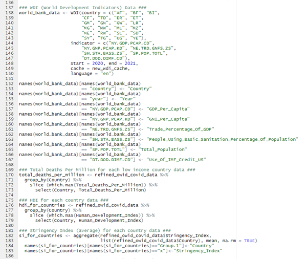
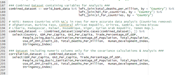
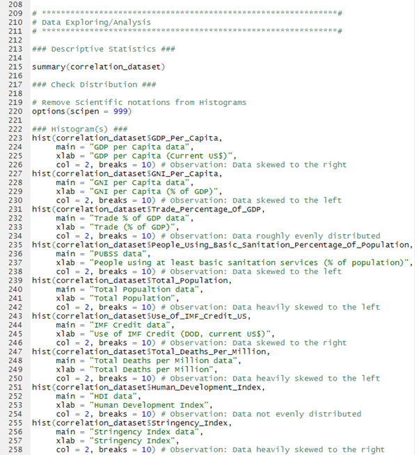
R Code:
References
Gupta, M., Wahl, B., Adhikari, B. et al. . (2020, 06 11). Global Health Research and Policy. The need for COVID-19 research in lowand middle-income countries, pp. 5-33.
Hannah Ritchie et al. (2021, January 27). Coronavirus Pandemic (COVID-19). Retrieved from OurWorldInData.org.: https://ourworldindata.org/coronavirus
Abel Brodeur et al. (2021). A literature review of the economics of. Journal of Economic Surveys, 1007-1009.
Shapiro, S., & Wilk, M. (1965). Biometrika. An analysis of variance test for normality (complete samples), 591-611.
O'Neil, C., & Schutt, R. (2014). Doing Data Science. Sebastopol: O'Reilly.
Tranmer, M., Murphy, J., Elliot, M., & Pampaka, M. (2020). Multiple Linear Regression. Cathie.
Rebekic, A., Loncaric, Z., Petrovic, S., & Maric, S. (2015). Pearson’s or spearman’s correlation coefficient – which one to. Poljoprivreda/Agriculture, 47-54.
Brown, S. H. (2009). Multiple Linear Regression Analysis: A Matrix Approach with. Alabama Journal of Mathematics, 1-3.
Tabachnick, B., & Fidell, S. (1996). Using Multivariate Statistics. New York: Harper Collins College.
Covid-19 Health System Response Monitor. (2022, January 29). HOW COMPARABLE IS COVID-19 MORTALITY ACROSS COUNTRIES?Retrieved from Covid-19 Health System Response Monitor: https://analysis.covid19healthsystem.org/index.php/2020/06/04/how-comparable-is-covid-19-mortality-across-countries/
Sannigrahi, S., Pilla, F., Basu, B., Basu, A., & Molter, A. (2020). Examining the association between socio-demographic composition and. Sustainable Cities and Society , 1-14.
Kauhl, B., Heil, J., J. P. A. Hoebe, C., Schweikart, J., Krafft, T., & H. T. M. Dukers-Muijrers, N. (2015). The Spatial Distribution of Hepatitis C Virus Infections and Associated Determinants—An Application of a Geographically Weighted Poisson Regression for Evidence-Based Screening Interventions in Hotspots. Plos One, 1-19.
Roecker, E. (1991). Prediction error and its estimation for subset—selected models. Technometrics, 459-468.
Stojkoski, V., Utkovski, Z., Jolakoski, P., Tevdovski, D., & Kocarev, L. (2020, November 17). The socio-economic determinants of the coronavirus. Cyril and Methodius University in Skopje, Faculty of Economics,.
Jay J H Park et al. (2021). How COVID-19 has fundamentally changed clinical research in global health. CLINICAL TRIALS IN GLOBAL HEALTH, 711-720.


Comments ()