Predicting Airline Passenger Satisfaction
Predicting airline passenger satisfaction with Knime analytics.

In this project for my MSc in Data Science I was tasked with predicting the target variable of Satisfaction ("satisfied" or "neutral or dissatisfied") from a variety of independent variables included in the Kaggle Airline Passenger Satisfaction Dataset. Utilising the swiss KNIME analytics platform which was built using Java, is free and open source.
Method(s):
Utilising the Airline Satisfaction Data and the KNIME Analytics Platform. Data exploration will be conducted to ascertain the relevant properties of the data, replace missing values, remove outliers, and remove any collinearity. Then two supervised models (Decision Tress and Naïve Bayes) were trained and then deployed on unseen data to predict the binary class membership of either satisfied/neutral or dissatisfied. Utilising performance measures (Confusion Matrix, Cohens Kappa and ROC Curves) evaluate and compare the different techniques performances and accuracy of there predictions.
Stage 1: Data Gathering
The dataset was provided by the university and downloaded as a .csv file which was then imported into KNIME with the file reader node. Pretty simple (for now).

Dataset variables:
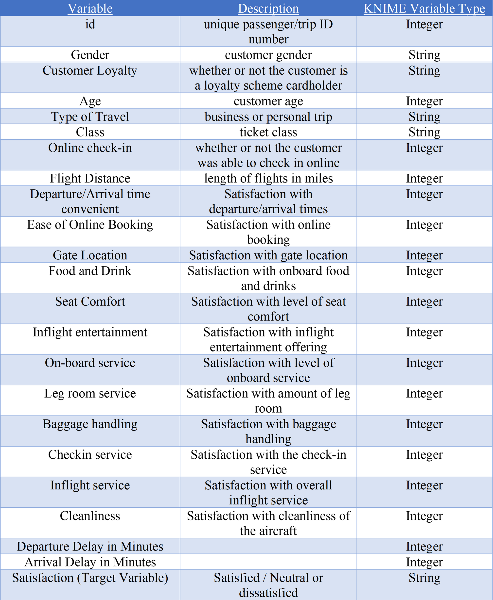
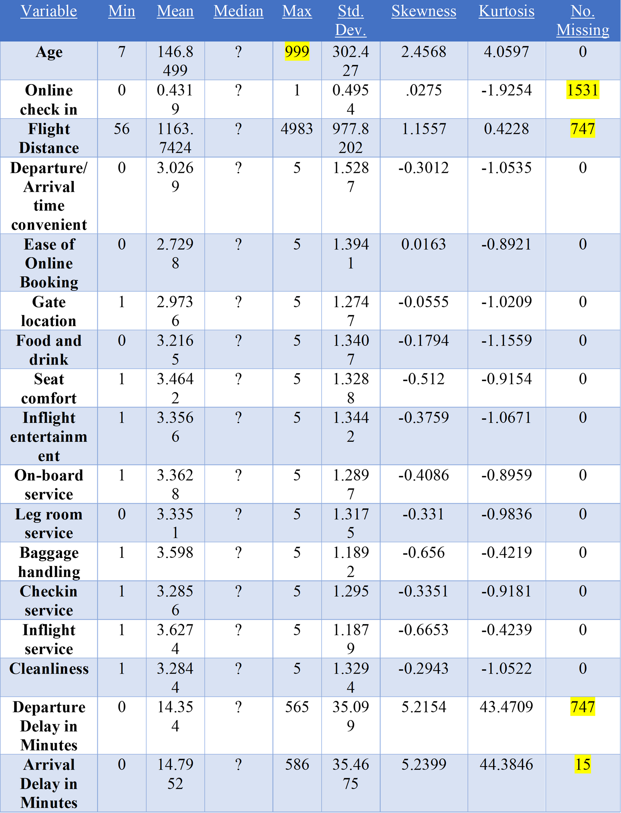
Then using the statistics node a variety of descriptive statistics were produced (see below) to gather more information about the data and to be used later in stage 3.

Summary Statistics:
Stage 2: Data Structuring
As identified above in the Summary Statistics, the online check in attribute had 1,531 missing values. This attribute was removed using the column filter node from the dataset. This many missing values did not add value to data or model with a pseudo value (if created) would make up more than 29% of the attribute.

Also, outliers of the age value were identified in the initial statistics node, showing people with maximum ages of 999, the row filter was used removing values pattern matching 999 to account for this outlier.

The missing values for flight distance were replaced with the average flight distance of the whole dataset with the missing value node, replacing 747 missing values.

This was then converted to an integer with the double to integer node.

The missing values for arrival and departure delays were replaced with the value 666 (this number was chosen as the maximum value in both attributes was 586, therefore when replaced would not affect any actual values in the data). Then two math formula nodes were deployed on each respective attribute, replacing the missing departure delay equal to 666 with the corresponding arrival delay replacing the missing arrival delay equal to 666 with the corresponding departure delay. This was performed as the variance between the distributions of both attributes was minimal.

Expression for replaced departure delay: if($Departure Delay in Minutes$ == 666, $Arrival Delay in Minutes$ , $Departure Delay in Minutes$).
Expression for replaced arrival delay: if($Arrival Delay in Minutes$ == 666, $Departure Delay in Minutes$ , $Arrival Delay in Minutes$)
For this dataset min-max normalisation was utilised. Min-max normalisation performs a linear alteration on the original data, with all the values falling between 0-1 (Saranya & Manikandan, 2013) which helps with distribution for the naïve bayes method, as mentioned previously this classification method relies on normal distribution of attributes.
Stage 3: Exploratory Data Analysis (EDA)
The following pie chart was created to show the overall percentages of customer satisfaction within the dataset. If the data is unbalanced this can lead to overtraining the data to predict one class of sentiment.
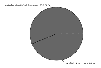
With the data not perfectly balanced the equal size sampling node was needed. To ensure that equal sizes of the binary target variable were used in training and test data.

Box plots were produced (see below) expressing the minimum, lower quartile, median, upper quartile, and maximum figures. This is useful for observing the features of nominal attributes and seeing if there is any overlap between the class instances.


Collinearity was also looked for in the variables as for the naïve bayes classification method it is assumed that all variables are independent of each other (Hastie, Tibshirani, & Friedman, 2009). This was done through the Linear Correlation Node.

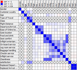
Observing the matrix, it is clear there is a strong relationship between the departure delay time and arrival delay time.
Experimental Setup
For technical details of the experimental setup please see below:
Feature Selections
A correlation filter node was applied to filter out all correlations equal to or greater than 0.8, this filtered out the arrival delay time feature as the correlation with the departure delay time was 0.9707.
The customer id attribute was removed (with the column filter node) as it did not add value and could lead to reduced performance of the classification method.
Equal Size Sampling
As seen in the Pie Chart of Customer Satisfaction Percentages, the dataset had an unbalanced set of the categorical class, this may lead to overfitting on a certain categorical class. The equal size sampling node was selected to equally distribute the nominal value of satisfaction, using exact sampling so that each class will have the same number of instances in the output table.
Partitioning
Many researchers propose an 80/20 training and testing set split for their datasets (Nguyen, et al., 2021). The 80% training data was created using stratified sampling so that the distribution of values was retained in the output tables, this partitioning ensures that none of the training data is used within the test data as this would invalidate results.
Cross Validation
Cross validation was applied, it is argued by (Murthy, 1998) that k = 10 is generally believed to be a “honest” assessment of tree predictive quality. This was applied to the training sets of both models to compare the performance, but also to see the effects on accuracy and Cohen’s kappa if the models were not put through cross validation. This was implemented with the x-partitioner node, all nodes between this and the x-aggregator node are executed 10 times. The x-aggregator node collects the results from the 10 iterations, comparing the predicted/real class and produces the predictions for all rows. Cross validation was performed as data was scarce and to ensure models were not overfitted.
Decision Tree
The decision tree learner node was used to produce a decision tree model for the airline satisfaction data, the class column selected was satisfaction as this is the target feature to be predicted. The quality measure used as stated in was the Gini Index to decide the best split for the decision tree nodes but also the information gain ratio was also selected for comparison. Pruning method was performed with and without MDL and binary nominal splits was selected as this is a binary classification problem of satisfied/neutral or dissatisfied. This was then connected to a decision tree predictor node to predict the class membership of the airline customers on unseen test data.
Naive Bayes
For the Naïve Bayes model, the naïve bayes learner node was used to create a Bayesian model from the training data, this was done for 10 iterations as it was utilised with the x-partitioner and x-aggregator node like with the decision tree model. The classification column was selected as satisfaction. Maximum number of unique nominal values per attribute was set to 20. This was then connected to a naïve bayes predictor node which predicted the class per row based on the Bayesian model produced earlier.
Evaluation Measures
The evaluation measures for model performance were the confusion matrix and accuracy statistics produced by the scorer node. This included a measure of accuracy of each model and the Cohens Kappa of each model. The results of which are discussed in the next section in further detail. Also, the choice of gain ratio or Gini index for deciding the splits in the decision tree was measured. ROC curves of each model were also produced for comparison.
Stage 4: Results and Discussion
The results of each model produced being deployed on the test data, with different parameters are displayed in table 7 & 8 below:
Decision Tree:

As see in the table Model 4 possessed the highest Cohens Kappa and Accuracy scores, this was applying the gain ratios for splits and applying the MDL pruning method. A confusion matrix for this model was produced below to compare against the naïve bayes classification method.

Naive Bayes:

Model 1 possessed the highest evaluation measure scores; it is worth noting that as the threshold standard deviation increased both performance measures decreased. See below for a confusion matrix of the naïve bayes model results.

Comparing the models:
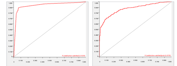
Overall, the Decision Tree Model 4 performed the best on the test data in both evaluation methods 0.91 Cohens Kappa compared to the Naïve Bayes model only achieving 0.71. Also, the decision tree model had highest accuracy of 0.82 whereas the Naïve Bayes model only had 0.59. With accuracy being an intuitive way of measuring performance of a classification model (Banihashemi, Ding, & Wang, 2017) it can be concluded that the decision tree is the more appropriate model. This may be because the assumption of independence with the naïve bayes model may not have been achieved with the correlation filter node of 0.8 however as (Ashari, Paryudi, & Tjoa, 2013) state the naïve bayes algorithm can/should preform without this independence. The ROC curves below show the two respective models performance in terms of AUC where a value of 0 shows a perfectly inaccurate test and a value of 1 reflects a perfectly accurate test (Mandrekar, 2010). Shown below in the ROC curves there is a 93.39% chance that the Decision tree model will accurately classify a customer. Whereas with the naïve bayes model there is only an 87.35% chance of an accurate classification.
The most notable attribute that classified the data in the decision tree method was whether the customers flew in business class or economy, with most people in business class satisfied and economy neutral or dissatisfied. This would make sense as business class usually has more comfort for customers charged at a higher price, whereas economy seats have less space.
Conclusion
In summary the decision tree was this more accurate model on the test data with an error rate of 8.765%, Accuracy of 0.82 and Cohens Kappa of 0.91. This may have surpassed the naïve bayes model due to the decision trees ability to handle a mix set of data types (Ashari, Paryudi, & Tjoa, 2013). The most important feature identified was the class of flight the customers travelled on (business or economy).
With hindsight “smoothing” of the data would’ve been applied for the naïve bayes model as the algorithm can fail if the attribute value does not occur in the training set in line with other classes and it will have no prior probability. This could have been applied to flight distance, age, and arrival/departure time delay.
Also, a validation set of the data may have complemented analysis by extracting a third sample from the dataset. Building the initial models on the training set and then using the validations set to choose parameters that that avoid overfitting. This split would have been 70/20/10 as suggested by (Nguyen, et al., 2021).
References
Hastie, T., Tibshirani, R., & Friedman, J. (2009). The Elements of Statistical Learning. New York: Springer.
Saranya, C., & Manikandan, G. (2013). A Study on Normalization Techniques for Privacy Preserving Data Mining. International Journal of Engineering and Technology (IJET), 2701-2704.
Nguyen, Q. H., Ly, H.-B., Ho, L. S., Al-Ansari, N., Van Le, H., Tran, V. Q., . . . Pham, B. T. (2021). Influence of Data Splitting on Performance of Machine Learning Models in Prediction of Shear Strength of Soi. Artificial Intelligence for Civil Engineering, 1024-1123.
Murthy, S. K. (1998). Automatic Construction of Decision Trees from Data: A Multi-Disciplinary Survey. Data Mining and Knowledge Discovery, 2,, 345-398.
Banihashemi, S., Ding, G., & Wang, J. (2017). "Developing a Hybrid Model of Prediction and Classification Algorithms for Building Energy Consumption. Energy Procedia, Vol.110,, 371-376.
Ashari, A., Paryudi, I., & Tjoa, A. (2013). Performance Comparison between Naïve Bayes, Decision Tree and k-Nearest Neighbor in Searching Alternative Design in an Energy Simulation Tool. (IJACSA) International Journal of Advanced Computer Science and Applications, 33-39.
Mandrekar, J. N. (2010). Receiver Operating Characteristic Curve in Diagnostic Test Assessment. BIOSTATISTICS FOR CLINICIANS, 1315-1316.


Comments ()